TL;DR: efficient secret sharing requires fast polynomial evaluation and interpolation; here we go through what it takes to use the well-known Fast Fourier Transform for this.
In the first part we looked at Shamir’s scheme, as well as its packed variant where several secrets are shared together. We saw that polynomials lie at the core of both schemes, and that implementation is basically a question of (partially) converting back and forth between two different representations of these. We also gave typical algorithms for doing this.
For this part we will look at somewhat more complex algorithms in an attempt to speed up the computations needed for generating shares. Specifically, we will implement and apply the Fast Fourier Transform, detailing all the essential steps. Performance measurements performed with our Rust implementation shows that this yields orders of magnitude of efficiency improvements when either the number of shares or the number of secrets is high.
There is also an associated Python notebook to better see how the code samples fit together in the bigger picture.
Polynomials
If we look back at Shamir’s scheme we see that it’s all about polynomials: a random polynomial embedding the secret is sampled and the shares are taken as its values at a certain set of points.
def shamir_share(secret):
    polynomial = sample_shamir_polynomial(secret)
    shares = [ evaluate_at_point(polynomial, p) for p in SHARE_POINTS ]
    return shares
The same goes for the packed variant, where several secrets are embedded in the sampled polynomial.
def packed_share(secrets):
    polynomial = sample_packed_polynomial(secrets)
    shares = [ interpolate_at_point(polynomial, p) for p in SHARE_POINTS ]
    return shares
Notice however that they differ slightly in the second steps where the shares are computed: Shamir’s scheme uses evaluate_at_point while the packed uses interpolate_at_point. The reason is that the sampled polynomial in the former case is in coefficient representation while in the latter it is in point-value representation.
Specifically, we often represent a polynomial f of degree D == L-1 by a list of L coefficients a0, ..., aD such that f(x) = (a0) + (a1 * x) + (a2 * x^2) + ... + (aD * x^D). This representation is convenient for many things, including efficiently evaluating the polynomial at a given point using e.g. Horner’s method.
However, every such polynomial may also be represented by a set of L point-value pairs (p1, v1), ..., (pL, vL) where vi == f(pi) and all the pi are distinct. Evaluating the polynomial at a given point is still possible, yet now requires a more involved interpolation procedure that may be less efficient.
But the point-value representation also has several advantages, most importantly that every element intuitively contributes with the same amount of information, unlike the coefficient representation where, in the case of secret sharing, a few elements are the actual secrets; this property gives us the privacy guarantee we are after. Moreover, a degree L-1 polynomial may also be represented by more than L pairs; in this case there is some redundancy in the representation that we may for instance take advantage of in secret sharing (to reconstruct even if some shares are lost) and in coding theory (to decode correctly even if some errors occur during transmission).
The reason this works is that the result of interpolation on a point-value representation with L pairs is technically speaking defined with respect to the least degree polynomial g such that g(pi) == vi for all pairs in the set, which is unique and has at most degree L-1. This means that if two point-value representations are generated using the same polynomial g then interpolation on these will yield identical results, even when the two sets are of different sizes or use different points, since the least degree polynomial is the same.
It is also why we can use the two representations somewhat interchangeably: if a point-value representation with L pairs where generated by a degree L-1 polynomial f, then the unique least degree polynomial agreeing with these must be f. And since, for a fixed set of points, the set of coefficient lists of length L and the set of value lists of length L has the same cardinality (in our case Q^L) we must have a bijection between them.
Fast Fourier Transform
With the two presentation of polynomials in mind we move on to how the Fast Fourier Transform (FFT) over finite fields – also known as the Number Theoretic Transform (NTT) – can be used to perform efficient conversion between them. And for me the best way of understanding this is through an example that can later be generalised into an algorithm.
Walk-through example
Recall that all our computations happen in a prime field determined by a fixed prime Q, i.e. using the numbers 0, 1, ..., Q-1. In this example we will use Q = 433, who’s order Q-1 is divisible by 4: Q-1 == 432 == 4 * k with k = 108.
Assume then that we have a polynomial A(x) = 1 + 2x + 3x^2 + 4x^3 over this field of with L == 4 coefficients and degree L-1 == 3.
A_coeffs = [ 1, 2, 3, 4 ]
Our goal is to turn this list of coefficients into a list of values [ A(w0), A(w1), A(w2), A(w3) ] of equal length, for points w = [w0, w1, w2, w3].
The standard way of evaluating polynomials is of course one way of during this, which using Horner’s rule can be done in a total of Oh(L * L) operations.
A = lambda x: horner_evaluate(A_coeffs, x)

assert([ A(wi) for wi in w ]
    == [ 10, 73, 431, 356 ])
But as we will see, the FFT allows us to do so more efficiently when the length is sufficiently large and the points are chosen with a certain structure; asymptotically we can compute the values in Oh(L * log L) operations.
The first insight we need is that there is an alternative evaluation strategy that breaks A into two smaller polynomials. In particular, if we define polynomials B(y) = 1 + 3y and C(y) = 2 + 4y by taking every other coefficient from A then we have A(x) == B(x * x) + x * C(x * x), which is straight-forward to verify by simply writing out the right-hand side.
This means that if we know values of B(y) and C(y) at the squares v of the w points, then we can use these to compute the values of A(x) at the w points using table look-ups: A_values[i] = B_values[i] + w[i] * C_values[i].
# split A into B and C
B_coeffs = A_coeffs[0::2] # == [ 1,    3,   ]
C_coeffs = A_coeffs[1::2] # == [    2,    4 ]

# square the w points
v = [ wi * wi % Q for wi in w ]

# somehow compute the values of B and C at the v points
# ...
assert( B_values == [ B(vi) for vi in v ] )
assert( C_values == [ C(vi) for vi in v ] )

# combine results into values of A at the w points
A_values = [ ( B_values[i] + w[i] * C_values[i] ) % Q for i,_ in enumerate(w) ]

assert( A_values == [ A(wi) for wi in w ] )
So far we haven’t saved much, but the second insight fixes that: by picking the points w to be the elements of a subgroup of order 4, the v points used for B and C will form a subgroup of order 2 due to the squaring; hence, we will have v[0] == v[2] and v[1] == v[3] and so only need the first halves of B_values and C_values – as such we have cut the subproblems in half!
Such subgroups are typically characterized by a generator, i.e. an element of the field that when raised to powers will take on exactly the values of the subgroup elements. Historically such generators are denoted by the omega symbol so let’s follow that convention here as well.
# generator of subgroup of order 4
omega4 = 179

w = [ pow(omega4, e, Q) for e in range(4) ]
assert( w == [1, 179, 432, 254] )
We shall return to how to find such generator below, but note that once we know one of order 4 then it’s easy to find one of order 2: we simply square.
# generator of subgroup of order 2
omega2 = omega4 * omega4 % Q

v = [ pow(omega2, e, Q) for e in range(2) ]
assert( v == [1, 432] )
As a quick test we may also check that the orders are indeed as claimed. Specifically, if we keep raising omega4 to higher powers then we except to keep visiting the same four numbers, and likewise we expect to keep visiting the same two numbers for omega2.
assert( [ pow(omega4, e, Q) for e in range(8) ] == [1, 179, 432, 254, 1, 179, 432, 254] )
assert( [ pow(omega2, e, Q) for e in range(8) ] == [1, 432,   1, 432, 1, 432,   1, 432] )
Using generators we also see that there is no need to explicitly calculate the lists w and v anymore as they are now implicitly defined by the generator. So, with these change we come back to our mission of computing the values of A at the points determined by the powers of omega4, which may then be done via A_values[i] = B_values[i % 2] + pow(omega4, i, Q) * C_values[i % 2].
The third and final insight we need is that we can of course continue this process of diving the polynomial in half: to compute e.g. B_values we break B into two polynomials D and E and then follow the same procedure; in this case D and E will be simple constants but it works in the general case as well. The only requirement is that the length L is a power of 2 and that we can find a generator omegaL of a subgroup of this size.
Algorithm for powers of 2
Putting the above into an algorithm we get the following, where omega is assumed to be a generator of order len(A_coeffs). Note that some typical optimizations are omitted for clarity (but see e.g. the Python notebook).
def fft2_forward(A_coeffs, omega):
    if len(A_coeffs) == 1:
        return A_coeffs

    # split A into B and C such that A(x) = B(x^2) + x * C(x^2)
    B_coeffs = A_coeffs[0::2]
    C_coeffs = A_coeffs[1::2]

    # apply recursively
    omega_squared = pow(omega, 2, Q)
    B_values = fft2_forward(B_coeffs, omega_squared)
    C_values = fft2_forward(C_coeffs, omega_squared)

    # combine subresults
    A_values = [0] * len(A_coeffs)
    L_half = len(A_coeffs) // 2
    for i in range(L_half):

        j = i
        x = pow(omega, j, Q)
        A_values[j] = (B_values[i] + x * C_values[i]) % Q

        j = i + L_half
        x = pow(omega, j, Q)
        A_values[j] = (B_values[i] + x * C_values[i]) % Q

    return A_values
With this procedure we may convert a polynomial in coefficient form to its point-value form, i.e. evaluate the polynomial, in Oh(L * log L) operations.
The freedom we gave up to achieve this is that the number of coefficients L must now be a power of 2; but of course, some of the them may be zero so we are still free to choose the degree of the polynomial as we wish up to L-1. Also, we are no longer free to choose any set of evaluation points but have to choose a set with a certain subgroup structure.
Finally, it turns out that we can also use the above procedure to go in the opposite direction from point-value form to coefficient form, i.e. interpolate the least degree polynomial. We see that this is simply done by essentially treating the values as coefficients followed by a scaling, but won’t go into the details here.
def fft2_backward(A_values, omega):
    L_inv = inverse(len(A_values))
    A_coeffs = [ (a * L_inv) % Q for a in fft2_forward(A, inverse(omega)) ]
    return A_coeffs
Here however we may feel a stronger impact of the constraints implied by the FFT: while we can use zero coefficients to “patch up” the coefficient representation of a lower degree polynomial to make its length match our target length L but keeping its identity, we cannot simply add e.g. zero pairs to a point-value representation as it may change the implicit least degree polynomial; as we will see in the next blog post this has implications for our application to secret sharing if we also want to use the FFT for reconstruction.
Algorithm for powers of 3
Unsurprisingly there is nothing in the principles behind the FFT that means it will only work for powers of 2, and other bases can indeed be used as well. Luckily perhaps, since this plays a big part in our application to secret sharing as we will see below.
To adapt the FFT algorithm to powers of 3 we instead assume that the list of coefficients of A has such a length, and split it into three polynomials B, C, and D such that A(x) = B(x^3) + x * C(x^3) + x^2 * D(x^3), and we use the cube of omega in the recursive calls instead of the square. Here omega is again assumed be a generator of order len(A_coeffs), but this time a power of 3.
def fft3_forward(A_coeffs, omega):
    if len(A_coeffs) == 1:
        return A_coeffs

    # split A into B, C, and D such that A(x) = B(x^3) + x * C(x^3) + x^2 * D(x^3)
    B_coeffs = A_coeffs[0::3]
    B_coeffs = A_coeffs[1::3]
    B_coeffs = A_coeffs[2::3]

    # apply recursively
    omega_cubed = pow(omega, 3, Q)
    B_values = fft3_forward(B_coeffs, omega_cubed)
    C_values = fft3_forward(B_coeffs, omega_cubed)
    D_values = fft3_forward(B_coeffs, omega_cubed)

    # combine subresults
    A_values = [0] * len(A_coeffs)
    L_third = len(A_coeffs) // 3
    for i in range(L_third):

        j  = i
        x  = pow(omega, j, Q)
        xx = pow(x, 2, Q)
        A_values[j] = (B_values[i] + x * C_values[i] + xx * D_values[i]) % Q

        j  = i + L_third
        x  = pow(omega, j, Q)
        xx = pow(x, 2, Q)
        A_values[j] = (B_values[i] + x * C_values[i] + xx * D_values[i]) % Q

        j  = i + L_third + L_third
        x  = pow(omega, j, Q)
        xx = pow(x, 2, Q)
        A_values[j] = (B_values[i] + x * C_values[i] + xx * D_values[i]) % Q

    return A_values
And again we may go in the opposite direction and perform interpolation by simply treating the values as coefficients and performing a scaling.
Optimizations
For easy of presentation we have omitted some typical optimizations here, perhaps most typically the fact that for powers of 2 we have the property that pow(omega, i, Q) == -pow(omega, i + L/2, Q), meaning we can cut the number of exponentiations in fft2 in half compared to what we did above.
More interestingly, the FFTs can be also run in-place and hence reusing the list in which the input is provided. This saves memory allocations and has a significant impact on performance. Likewise, we may gain improvements by switching to another number representation such as Montgomery form. Both of these approaches are described in further detail elsewhere.
Application to Secret Sharing
We can now return to applying the FFT to the secret sharing schemes. As mentioned earlier, using this instead of the more traditional approaches makes most sense when the vectors we are dealing with are above a certain size, such as if we are generating many shares or sharing many secrets together.
Shamir’s scheme
In this scheme we can easily sample our polynomial directly in coefficient representation, and hence the FFT is only relevant in the second step where we generate the shares. Concretely, we can directly sample the polynomial with the desired number of coefficients to match our privacy threshold, and add extra zeros to get a number of coefficients matching the number of shares we want; below the former list is denoted as small and the latter as large. We then apply the forward FFT to turn this into a list of values that we take as the shares.
def shamir_share(secret):
    small_coeffs = [secret] + [random.randrange(Q) for _ in range(T)]
    large_coeffs = small_coeffs + [0] * (ORDER_LARGE - len(small_coeffs))
    large_values = fft3_forward(large_coeffs, OMEGA_LARGE)
    shares = large_values
    return shares
Besides the privacy threshold T and the number of shares N, the parameters needed for the scheme is hence a prime Q and a generator OMEGA_LARGE of order ORDER_LARGE == N + 1.
Note that we’ve used the FFT for powers of 3 here to be consistent with the next scheme; the FFT for powers of 2 would of course also have worked.
Packed scheme
Recall that for this scheme it is less obvious how we can sample our polynomial directly in coefficient representation, and hence we instead do so in point-value representation. Specifically, we first use the backward FFT for powers of 2 to turn such a polynomial into coefficient representation, and then as above use the forward FFT for powers of 3 on this to generate the shares.
We are hence dealing with two sets of points: those used during sampling, and those used during share generation – and these cannot overlap! If they did the privacy guarantee would no longer be satisfied and some of the shares might literally equal some of the secrets.
Preventing this from happening is the reason we use the two different bases 2 and 3: by picking co-prime bases, i.e. gcd(2, 3) == 1, the subgroups will only have the point 1 in common (as the two generators raised to the zeroth power). As such we are safe if we simply make sure to exclude the value at point 1 from being used. Recalling our walk-through example, this is the reason we used prime Q == 433 since its order Q-1 == 432 == 4 * 9 * k is divided by both a power of 2 and a power of 3.
So to do sharing we first sample the values of the polynomial, fixing the value at point 1 to be a constant (in this case zero). Using the backward FFT we then turn this into a small list of coefficients, which we then as in Shamir’s scheme extend with zero coefficients to get a large list of coefficients suitable for running through the forward FFT. Finally, since the first value obtained from this corresponds to point 1, and hence is the same as the constant used before, we remove it before returning the values as shares.
def packed_share(secrets):
    small_values = [0] + secrets + [random.randrange(Q) for _ in range(T)]
    small_coeffs = fft2_backward(small_values, OMEGA_SMALL)
    large_coeffs = small_coeffs + [0] * (ORDER_LARGE - ORDER_SMALL)
    large_values = fft3_forward(large_coeffs, OMEGA_LARGE)
    shares = large_values[1:]
    return shares
For this scheme, besides T, N, and the number K of secrets packed together, the parameters for this scheme is hence the prime Q and the two generators OMEGA_SMALL and OMEGA_LARGE of order respectively ORDER_SMALL == T + K + 1 and ORDER_LARGE == N + 1.
We will talk more about how to do efficient reconstruction in the next blog post, but note that if all the shares are known then the above sharing procedure can efficiently be run backwards by simply running the two FFTs in their opposite direction.
def packed_reconstruct(shares):
    large_values = [0] + shares
    large_coeffs = fft3_backward(large_values, OMEGA_LARGE)
    small_coeffs = large_coeffs[:ORDER_SMALL]
    small_values = fft2_forward(small_coeffs, OMEGA_SMALL)
    secrets = small_values[1:K+1]
    return secrets
However this only works if all shares are known and correct: any loss or tampering will get in the way of using the FFT for reconstruction, unless we add an additional ingredient. Fixing this is the topic of the next blog post.
Performance evaluation
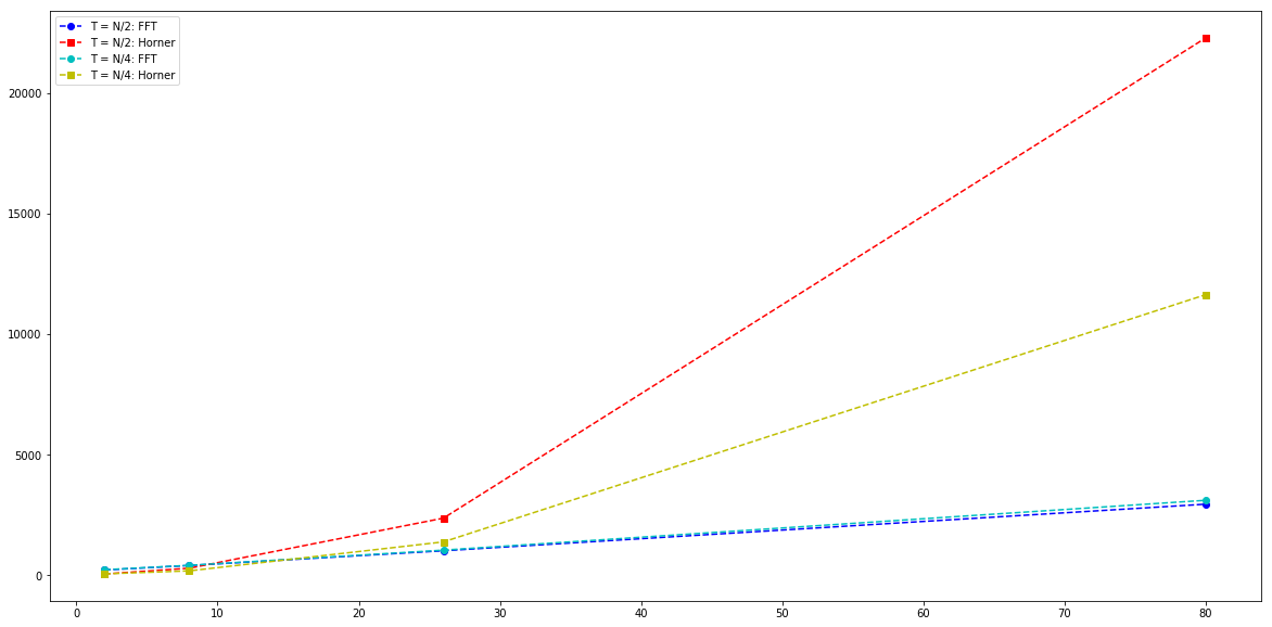
To test the performance impact of using the FFT for share generation in Shamir’s scheme, we let the number of shares N take on values 2, 8, 26, 80 and 242, and for each of them compare against the typical approach of using Horner’s rule. For the former we have an asymptotic complexity of Oh(N * log N) while for the latter we have Oh(N * T), and as such it is also interesting to vary T; we do so with T = N/2 and T = N/4, representing respectively a medium and low privacy threshold.
All measures are in nanoseconds (1/1,000,000 milliseconds) and performed with our Rust implementation.
plt.figure(figsize=(20,10))

shares    = [   2,   8,   26,    80 ] #,    242 ]

n2_fft    = [ 214, 402, 1012,  2944 ] #,  10525 ]
n2_horner = [  51, 289, 2365, 22278 ] #, 203630 ]

n4_fft    = [ 227, 409, 1038,  3105 ] #,  10470 ]
n4_horner = [  54, 180, 1380, 11631 ] #, 104388 ]

plt.plot(shares, n2_fft,    'ro--', color='b', label='T = N/2: FFT')
plt.plot(shares, n2_horner, 'rs--', color='r', label='T = N/2: Horner')
plt.plot(shares, n4_fft,    'ro--', color='c', label='T = N/4: FFT')
plt.plot(shares, n4_horner, 'rs--', color='y', label='T = N/4: Horner')

plt.legend(loc=2)
plt.show()
Note that the numbers for N = 242 are omitted in the graph to avoid hiding the results for the smaller values.
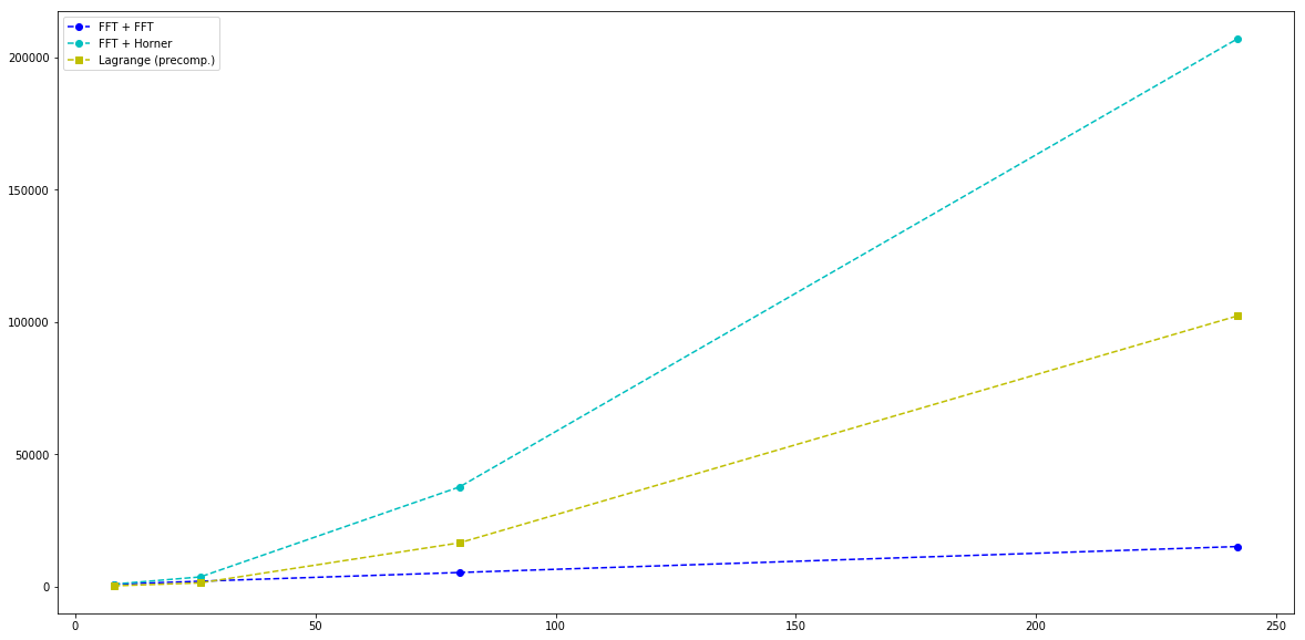
For the packed scheme we keep T = N/4 and K = N/2 fixed (meaning R = 3N/4) and let N vary as above. We then compare three different approaches for generating shares, all starting out with sampling a polynomial in point-value representation:
FFT + FFT: Backward FFT to convert into coefficient representation, followed by forward FFT for evaluationFFT + Horner: Backward FFT to convert into coefficient representation, followed by Horner’s rule for evaluationLagrange: Use precomputed Lagrange constants for share points to directly obtain shares
where the third option requires additional storage for the precomputed constants (computing them on the fly increases the running time significantly but can of course be amortized away if processing a large number of batches).
plt.figure(figsize=(20,10))

shares =       [    8,   26,    80,    242 ]

fft_fft      = [  840, 1998,  5288,  15102 ]
fft_horner   = [  898, 3612, 37641, 207087 ]
lagrange_pre = [  246, 1367, 16510, 102317 ]

plt.plot(shares, fft_fft,      'ro--', color='b', label='FFT + FFT')
plt.plot(shares, fft_horner,   'ro--', color='r', label='FFT + Horner')
plt.plot(shares, lagrange_pre, 'rs--', color='y', label='Lagrange (precomp.)')

plt.legend(loc=2)
plt.show()
We note that the Lagrange approach remains superior up to the setting with 26 shares, after which it’s interesting to use the two step FFT.
From this small amount of empirical data the FFT seems like the obvious choice as soon as the number of shares is sufficiently high. Question of course, is in which applications this is the case. We will explore this further in a future blog post (or see e.g. our paper).
Parameter Generation
Since there are no security implications in re-using the same fixed set of parameters (i.e. Q, OMEGA_SMALL, and OMEGA_LARGE) across applications, parameter generation is perhaps less important compared to for instance key generation in encryption schemes. Nonetheless, one of the benefits of secret sharing schemes is their ability to avoid big expansion factors by using parameters tailored to the use case; concretely, to pick a field of just the right size. As such we shall now fill in this final piece of the puzzle and see how a set of parameters fitting with the FFTs used in the packed scheme can be generated.
Our main abstraction is the generate_parameters function which takes a desired minimum field size in bits, as well as the number of secrets k we which to packed together, the privacy threshold t we want, and the number n of shares to generate. Accounting for the value at point 1 that we are throwing away (see earlier), to be suitable for the two FFTs, we must then have that k + t + 1 is a power of 2 and that n + 1 is a power of 3.
To next make sure that our field has two subgroups with those number of elements, we simply need to find a field whose order is divided by both numbers. Specifically, since we’re considering prime fields, we need to find a prime q such that its order q-1 is divided by both sizes. Finally, we also need a generator g of the field, which can be turned into generators omega_small and omega_large of the subgroups.
def generate_parameters(min_bitsize, k, t, n):
    order_small = k + t + 1
    order_large = n + 1

    order_divisor = order_small * order_large
    q, g = find_prime_field(min_bitsize, order_divisor)

    order = q - 1
    omega_small = pow(g, order // order_small, q)
    omega_large = pow(g, order // order_large, q)

    return q, omega_small, omega_large
Finding our q and g is done by find_prime_field, which works by first finding a prime of the right size and with the right order. To then also find the generator we need a piece of auxiliary information, namely the prime factors in the order.
def find_prime_field(min_bitsize, order_divisor):
    q, order_prime_factors = find_prime(min_bitsize, order_divisor)
    g = find_generator(q, order_prime_factors)
    return q, g
The reason for this is that we can use the prime factors of the order to efficiently test whether an arbitrary candidate element in the field is in fact a generator with that order. This follows from Lagrange’s theorem as detailed in standard textbooks on the matter.
def find_generator(q, order_prime_factors):
    order = q - 1
    for candidate in range(2, q):
        for factor in order_prime_factors:
            exponent = order // factor
            if pow(candidate, exponent, q) == 1:
                break
        else:
            return candidate
This leaves us with only a few remaining question regarding finding prime numbers as explained next.
Finding primes
To find a prime q with the desired structure (i.e. of a certain minimum size and whose order q-1 has a given divisor) we may either do rejection sampling of primes until we hit one that satisfies our need, or we may construct it from smaller parts so that it by design fits with what we need. The latter appears more efficient so that is what we will do here.
Specifically, given min_bitsize and order_divisor we will do rejection sampling over two values k1 and k2 until q = k1 * k2 * order_divisor + 1 is a probable prime. The k1 is used to ensure that the minimum size is met, and k2 is used to give us a bit of wiggle room – it can in principle be omitted, but empirical tests show that it doesn’t have to be very large it give an efficiency boost, at the expense of potentially overshooting the desired field size by a few bits. Finally, since we also need to know the prime factorization of q - 1, and since this in general is believed to be an inherently slow process, we by construction ensure that k1 is a prime so that we only have to factor k2 and order_divisor, which we assume to be somewhat small and hence doable.
def find_prime(min_bitsize, order_divisor):
    while True:
        k1 = sample_prime(min_bitsize)
        for k2 in range(128):
            q = k1 * k2 * order_divisor + 1
            if is_prime(q):
                order_prime_factors  = [k1]
                order_prime_factors += prime_factor(k2)
                order_prime_factors += prime_factor(order_divisor)
                return q, order_prime_factors
Sampling primes are done using a standard randomized primality test.
def sample_prime(bitsize):
    lower = 1 << (bitsize-1)
    upper = 1 << (bitsize)
    while True:
        candidate = random.randrange(lower, upper)
        if is_prime(candidate):
            return candidate
And factoring a number is done by simply trying a fixed set of all small primes in sequence; this will of course not work if the input is too large, but that is not likely to happen in real-world applications.
def prime_factor(x):
    factors = []
    for prime in SMALL_PRIMES:
        if prime > x: break
        if x % prime == 0:
            factors.append(prime)
            x = remove_factor(x, prime)
    assert(x == 1)
    return factors
Putting these pieces together we end up with an efficient procedure for generating parameters for use with FFTs: finding large fields of size e.g. 128bits is a matter of milliseconds.
Next Steps
While we have seen that the Fast Fourier Transform can be used to greatly speed up the sharing process, it has a serious limitation when it comes to speeding up the reconstruction process: in its current form it requires all shares to be present and untampered with. As such, for some applications we may be forced to resort to the more traditional and slower approaches of Newton or Laplace interpolation.
In the next blog post we will look at a technique for also using the Fast Fourier Transform for reconstruction, using techniques from error correction codes to account for missing or faulty shares, yet get similar speedup benefits to what we achieved here.